Python - kappa4 Verteilung in der Statistik
scipy.stats.kappa4() ist eine kontinuierliche Zufallsvariable von Kappa 4, die mit einem Standardformat und einigen Formparametern definiert wird, um ihre Spezifikation zu vervollständigen. Die Wahrscheinlichkeitsdichte wird in der Standardform definiert und die Parameter loc und scale werden verwendet, um die Verteilung zu verschieben und / oder zu skalieren.
Parameter:
q: untere und obere Schwanzwahrscheinlichkeit
x: Quantile
loc: [optional] Standortparameter. Standard = 0
Skala: [optional] Skalierungsparameter. Standard = 1
Größe: [Tupel von Ints, optional] Form oder zufällige Variablen.
Momente: [optional] bestehend aus Buchstaben ['mvsk']; 'm' = Mittelwert, 'v' = Varianz, 's' = Fisher's Skew und 'k' = Fisher's Kurtosis. (Standard = 'mv').Ergebnisse: kontinuierliche kappa4-Zufallsvariable
Code 1: Erstellen einer kontinuierlichen Zufallsvariablen von kappa4
fromscipy.statsimportkappa4numargs=kappa4.numargsa, b=4.32,3.18rv=kappa4(a, b)("RV : \n", rv)
Ausgabe :
Wohnmobil:
 scipy.stats._distn_infrastructure.rv_frozen Objekt bei 0x000002A9D50D62C8
Code Nr. 2: Johnson SU kontinuierliche Variablen und Wahrscheinlichkeitsverteilung
importnumpy as npquantile=np.arange (0.01,1,0.1)R=kappa4.rvs(a, b, scale=2, size=10)("Random Variates : \n", R)
Ausgabe :
Zufällige Variablen:
 [0,62293659 0,62825781 0,62377628 0,62308697 0,62665555 0,62802109
 0,62872844 0,62728058 0,62679381 0,62297679]
Code 3: Grafische Darstellung.
importnumpy as npimportmatplotlib.pyplot as pltdistribution=np.linspace(0, np.minimum(rv.dist.b,3))("Distribution : \n", distribution)plot=plt.plot(distribution, rv.pdf(distribution))
Ausgabe :
Verbreitung:
 [0. 0,06122449 0,12244898 0,18367347 0,24489796 0,30612245
 0,36734694 0,42857143 0,48979592 0,55102041 0,6122449 0,67346939
 0,73469388 0,79591837 0,85714286 0,91836735 0,97959184 1,04081633
 1.10204082 1.16326531 1.2244898 1.28571429 1.34693878 1.40816327
 1.46938776 1.53061224 1.59183673 1.65306122 1.71428571 1.7755102
 1,83673469 1,89795918 1,95918367 2,02040816 2,08163265 2,14285714
 2.20408163 2.26530612 2.32653061 2.3877551 2.44897959 2.51020408
 2,57142857 2,63265306 2,69387755 2,75510204 2,81632653 2,87755102
 2.93877551 3.]
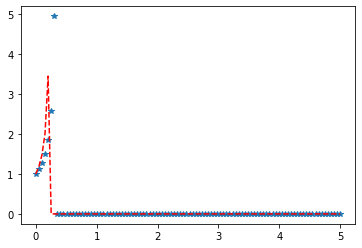
Code 4: Unterschiedliche Positionsargumente
importmatplotlib.pyplot as pltimportnumpy as npx=np.linspace(0,5,100)y1=kappa4 .pdf(x,1,3)y2=kappa4 .pdf(x,1,4)plt.plot(x, y1,"*", x, y2,"r--")
Ausgabe :