Python – Laplace-Verteilung in der Statistik
scipy.stats.laplace() ist eine kontinuierliche Laplace-Zufallsvariable. Es wird von den generischen Methoden als Instanz der Klasse rv_continuous geerbt . Es vervollständigt die Methoden mit Details, die für diese bestimmte Distribution spezifisch sind.
Parameter:
q : untere und obere Randwahrscheinlichkeit
x : Quantile
loc : [optionaler]Positionsparameter. Standard = 0
scale : [optional]scale-Parameter. Standard = 1
Größe : [Tupel von Ints, optional] Form oder zufällige Varianten.
Momente : [optional] zusammengesetzt aus Buchstaben ['mvsk']; 'm' = Mittelwert, 'v' = Varianz, 's' = Fisher's Schiefe und 'k' = Fisher's Kurtosis. (Standard = 'mv').Ergebnisse: Laplace-kontinuierliche Zufallsvariable
Code Nr. 1: Erstellen einer kontinuierlichen Laplace-Zufallsvariable
# importing library

from scipy.stats import laplace

numargs = laplace.numargs
a, b = 4.32, 3.18
rv = laplace(a, b)

print ("RV : \n", rv)
Ausgabe :
RV :
 scipy.stats._distn_infrastructure.rv_frozen object at 0x000002A9D4DAF708
Code Nr. 2: Laplace-kontinuierliche Varianzen und Wahrscheinlichkeitsverteilung
import numpy as np
quantile = np.arange (0.01, 1, 0.1)

# Random Variates
R = laplace.rvs(a, b)
print ("Random Variates : \n", R)

# PDF
R = laplace.pdf(a, b, quantile)
print ("\nProbability Distribution : \n", R)
Ausgabe :
Random Variates :
 10.613266250400734

Probability Distribution :
 [1.54667501e-48 1.43452207e-04 1.04508615e-02 4.07873394e-02
 7.56198196e-02 1.04863398e-01 1.26475923e-01 1.41381881e-01
 1.51096956e-01 1.56988338e-01]
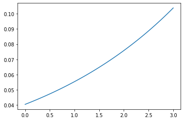
Code Nr. 3: Grafische Darstellung.
import numpy as np
import matplotlib.pyplot as plt

distribution = np.linspace(0, np.minimum(rv.dist.b, 3))
print("Distribution : \n", distribution)

plot = plt.plot(distribution, rv.pdf(distribution))
Ausgabe :
Distribution :
 [0.         0.06122449 0.12244898 0.18367347 0.24489796 0.30612245
 0.36734694 0.42857143 0.48979592 0.55102041 0.6122449  0.67346939
 0.73469388 0.79591837 0.85714286 0.91836735 0.97959184 1.04081633
 1.10204082 1.16326531 1.2244898  1.28571429 1.34693878 1.40816327
 1.46938776 1.53061224 1.59183673 1.65306122 1.71428571 1.7755102
 1.83673469 1.89795918 1.95918367 2.02040816 2.08163265 2.14285714
 2.20408163 2.26530612 2.32653061 2.3877551  2.44897959 2.51020408
 2.57142857 2.63265306 2.69387755 2.75510204 2.81632653 2.87755102
 2.93877551 3.        ]
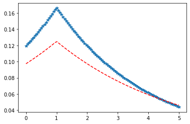
Code Nr. 4: Unterschiedliche Positionsargumente
import matplotlib.pyplot as plt
import numpy as np

x = np.linspace(0, 5, 100)

# Varying positional arguments
y1 = laplace .pdf(x, 1, 3)
y2 = laplace .pdf(x, 1, 4)
plt.plot(x, y1, "*", x, y2, "r--")
Ausgabe :